Analysis and Modeling: Machine Learning (SVM & RF) for RS Image Classification

For a PDF version of the paper click here

1   Introduction #

In the era of big data, the amount and availability of remote sensing and earth observation (EO) data as a whole has seen a large increase (Culberg & Fuhs, 2017; Lv & Wang, 2020). This increase stems not only from the larger quantity of imagery being captured but also from improvements to the spatial and spectral resolution of remote sensing images (Lv & Wang, 2020). A key aspect in the domain of remote sensing is obtaining meaningful information from the captured data. To achieve this, images are often classified. Classification of remote sensing images transforms raw pixel values of the earth’s surface, environment, and atmosphere into usable information by identifying and categorizing pieces of the image (Lv & Wang, 2020). This extraction of information by means of classification may be the end product or just an intermediate step of an analysis. Nonetheless, it is a crucial task to be performed (Thanh Noi & Kappas, 2017). Because of the large amount of generated data and because classifying images manually takes a great amount of time and effort, performant solutions are necessary. Following the stance that probabilistic methods are well suited to facilitate data analysis (Murphy, 2012), many methods of image classification with varying degrees of automation have been developed. These methods rely on the concept of machine learning.

The term machine learning is broad and contains many subcategories, encompassing many methods and individual approaches. It is classically split into the two main branches of predictive/supervised learning and descriptive/unsupervised learning (Murphy, 2012). While the task of image classification may make use of unsupervised methods (e.g., K-means clustering) to describe the data, supervised methods are the more commonly employed (Murphy, 2012). Two very popular supervised image classification methods focused on in this paper are the Support Vector Machine (SVM) and Random Forest (RF) classifiers. Thanh Noi & Kappas (2017) note a significant increase in the popularity of machine learning as a whole for remote-sensing-based applications between the years 2007 and 2017. Especially SVM and RF classification saw increased usage during this time span.

When employing these classical machine learning techniques, the image is analyzed based on its pixel values. Spatial topological relationships are not taken into account like in the more recently developed GEOBIA approach (Lang et al., 2019).

In recent years the concept of deep learning has shown impressive performance in many fields and may be one of the first things associated with machine learning. However, SVM and RF classifiers have distinct advantages over more complex deep learning approaches. The simpler design of these methods usually makes the results easier to interpret and explain. SVM and RF classifiers have also achieved good results on limited amounts of training data (Mahesh et al., 2022). Furthermore, these classifiers typically require significantly less computing power than most deep learning approaches.

This project employs the SVM and RF algorithms to perform land cover classification of multispectral Sentinel-2 imagery of San Marino. This study area can be seen in Figure 1. Two target land cover classifications are explored: the CORINE Land Cover (Büttner et al., 2021) provided by the Copernicus Land Monitoring service and a simplified land cover comprising three classes. Finally, an accuracy assessment is performed to validate the results.

2   Methods #

2.1   SVM #

The SVM algorithm was initially created by Cortes & Vapnik (1995) to perform binary classification of a dataset using labeled training data as input. The SVM is an extension of the maximal margin classifier and support vector classifier (also called soft margin classifier), unlike which it has the ability to classify data with non-linear class boundaries (James et al., 2021). The initial concept of the SVM can be further extended to allow for the classification of more than two classes. SVMs have been known to achieve high performance in various fields without requiring extensive modification to the algorithm (James et al., 2021; Mammone et al., 2009). This includes image classification in the field of EO. Culberg & Fuhs (2017) successfully demonstrate the automation of satellite imagery classification using the SVM and logistic regression models. Kranjčić et al. (2019) investigate the use of SVMs to classify green urban areas using Sentinel-2 imagery. The authors are able to achieve a high classification accuracy for two study areas (Kappa index = 0.87 and 0.89). Tzotsos (2006) evaluates the use of SVMs for object-based image classification of EO imagery with promising results.

The aim of the SVM is to find a suitable separation of data in a high-dimensional feature space, where each dimension represents a feature or characteristic of the data (Mammone et al., 2009). The initial data provided to the algorithm is labeled with the correct class. In the case of EO data, the features may be spectral reflectance values for which the label may be a certain landcover type. The two classes are separated by a threshold, commonly known as the hyperplane, which divides the feature space into two sections (in the case of binary classification). Each section corresponds to a separate class. The term hyperplane can be used to describe the separating threshold between two classes regardless of dimensionality. The dimensionality of the hyperplane is defined by the dimensionality of the feature space. In an \(n\)-dimensional feature space the hyperplane is \(n-1\) dimensions (James et al., 2021). If the feature space is 1-dimensional the hyperplane can also be referred to as a point. If the feature space is 2-dimensional the hyperplane is also a line. If the feature space is 3-dimensional the hyperplane is also plane. If the dimensions of the feature space are greater than 3 the hyperplane is simply described as a hyperplane (James et al., 2021).

The margin is defined as the shortest distance between the samples of each class and the hyperplane. An optimal hyperplane lies between the maximum margin (James et al., 2021; Mammone et al., 2009; Meyer, 2009). SVMs may employ different techniques to find the optimal margin. The maximal margin classifier can be used to find the maximum margin between two classes by placing the hyperplane between the closest data points of the two classes, regardless of data distribution. This technique is highly sensitive to outliers (poor model of real class distribution when the hyperplane placement is defined by outliers) and cannot be used for non-linearly separable data (James et al., 2021; Mammone et al., 2009). The support vector classifier can be used to create a more robust classification not susceptible to outliers by allowing for misclassifications (Mammone et al., 2009). The support vector classifier employs cross-validation of the data samples to find the optimal margin. The soft margin may result in samples of a class appearing on the wrong side of the hyperplane (misclassification) but represents the overall data distribution more accurately. When using a soft margin, the samples on the edge of the margin are referred to as support vectors (James et al., 2021).

While support vector classifiers allow for some overlap of the data, they cannot effectively classify non-linearly separable data. SVMs are able to do this by using kernels to (usually) add one or more additional dimensions to the feature space making the data linearly separable. A support vector classifier can then be found to separate the data into two groups (James et al., 2021; Meyer, 2009). The polynomial, radial basis function (RBF), and Gaussian kernels are among the most widely used (James et al., 2021; Lv & Wang, 2020; Thanh Noi & Kappas, 2017).

Once a suitable margin has been established, new data samples can be classified based on their feature values. This is done by checking on which side of the hyperplane the sample lies and assigning it to the appropriate class.

The use of a single SVM is inherently tied to binary classification, as the concept does not work well with more than two classes \(K\) (James et al., 2021). However, SVM classification may still be used to classify multiple classes. Two popular methods are one-versus-one (OVO) and one-versus-all (OVA) classification (James et al., 2021). These methods use different approaches to transform a multi-class classification into a series of binary classifications. For \(K>2\) classes, OVO classification creates an SVM for each pair of classes and performs a binary classification. When classifying a new sample, the number of times the sample is assigned to a certain class is noted. Finally, the sample is classified as the class to which it was assigned the most (James et al., 2021). This method shows similarities to the ensemble principle of the RF algorithm. The number of SVMs to be created can be expressed by the binomial coefficient of \(K\choose 2\), which potentially makes this method highly computationally intensive. Using OVO classification for five classes a total of 10 SVMs would be needed. For 10 classes a total of 45 SVMs would already be needed.

For \(K>2\) classes, OVA classification only trains as many SVMs as there are classes. Each SVM performs the classification for a certain class for which all other classes are treated as a single class, thus creating a binary classification. To classify a new sample, the sample is classified by each SVM. Since the sample is likely to be assigned to multiple classes during this process, the distance from the hyperplane is used as a confidence criterion. The greater the distance, the more likely it is to belong to that class. The sample is classified as the class for which it is the furthest from the hyperplane. An advantage of the OVA approach is the comparatively low number of SVMs needed.

2.2   Random Forest Classifier #

The random forest classifier is an ensemble method, meaning it is made up of many simple models. In this case decision trees. On their own, these simple models are not very accurate (Hastie et al., 2009). However, when combined, the resulting model can be very powerful (Belgiu & Drăgu, 2016; James et al., 2021). Similarly to the SVM, the RF algorithm is also commonly implemented to classify EO data. Rodriguez-Galiano et al. (2012) explore the performance of the RF algorithm for land cover classification of a complex area primarily using Landsat-5 data. The authors are able to achieve an overall classification accuracy of 92% (Kappa index = 0.92) with the RF algorithm outperforming a single decision tree model. Du et al. (2015) explore the use of ensemble methods for Polarimetric Synthetic Aperture Radar (PolSAR) image classification. Using textural features, morphological profiles, and polarimetric features the RF classifier is able to successfully classify images achieving similar performance to the benchmark SVM classifier. Pal (2005) describes the overall performance of the RF algorithm to also be comparable to that of the SVM for land cover classification.

The first step of the RF classifier creates multiple bootstrapped datasets from the original dataset (Hastie et al., 2009). Samples are randomly selected from the dataset and placed into a new dataset. The same sample may be selected more than once and others not at all. In this case the use of bootstrapping and then using the aggregate aims to reduce the variance of the classification and avoid overfitting of the model. Bootstrap aggregation is also known as bagging (James et al., 2021; Murphy, 2012).

Secondly, a decision tree is created for each bootstrapped dataset. In this process, only a subset of all features is used as candidates for the root node of the tree. The optimum number of subset features is calculated and the features themselves are selected randomly (Hastie et al., 2009). Among the subset, the best feature is selected as the root node and the node is split into two intermediate nodes. The process of selecting the best feature from the previously defined subset size and all following steps are repeated for all intermediate nodes until the minimum node size is reached and the tree is complete (Hastie et al., 2009).

Using the above steps, an ensemble of decision trees is created. The use of only a subset of all available features at each step ensures that single trees of the ensemble are less similar to each other, as otherwise the best predicting feature(s) would more frequently be chosen as nodes (James et al., 2021).

To classify a new data sample using the random forest method, the sample is given to each decision tree in the ensemble and the output of each tree is noted as a vote. The class with the highest number of votes is used as the final classification for the sample (Hastie et al., 2009).

Since samples can be chosen multiple times in the bootstrapped datasets, not every sample must be included. In practice, about one-third of the original samples are left out in each bootstrapped set (Breiman, 2001). These samples are called out-of-bag (OOB) samples and can be used to test the performance of each tree for which the sample is OOB. The proportion of all incorrectly classified OOB samples is called the OOB error. Using the OOB error as a measure of performance, the number of subset features to be selected as candidate nodes can be optimized by comparing the error for different values (Hastie et al., 2009; James et al., 2021).

2.3   Data #

2.3.1   Land Cover #

Two different land cover classifications are used as reference/ground truth classifications in this project. The first is the CORINE (Coordination of Information on the Environment) Land Cover (CLC) provided by the Copernicus Land Monitoring Service (Büttner et al., 2021). This database aims to be used as a standard for describing land cover in Europe to support environmental policy development (Büttner et al., 2021). In this project, the latest version of the database from 2018 is used. CLC classification is based on satellite and in-situ data. The CLC includes a total of 48 classes, of which the following 11 are present in the study area (Figure 2):

• Discontinuous urban fabric
• Industrial or commercial units
• Sport and leisure facilities
• Non-irrigated arable land
• Pastures
• Complex cultivation patterns
• Land principally occupied by agriculture, with significant areas of natural vegetation
• Broad-leaved forest
• Mixed forest
• Natural grasslands
• Transitional woodland-shrub.

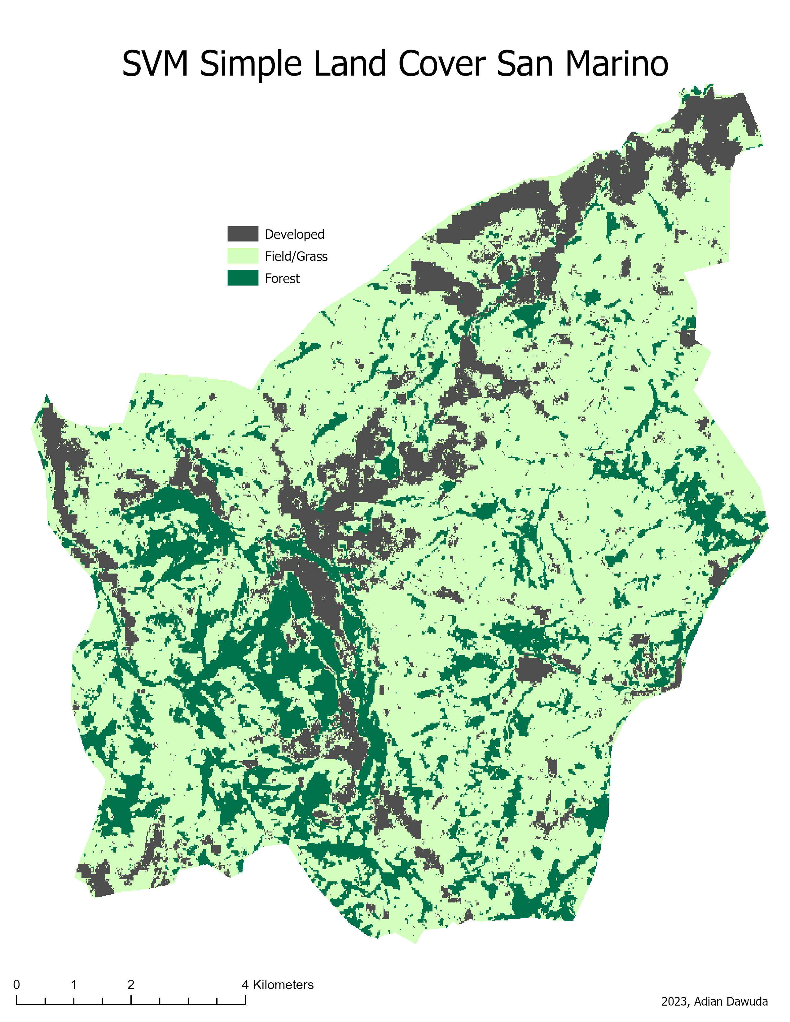
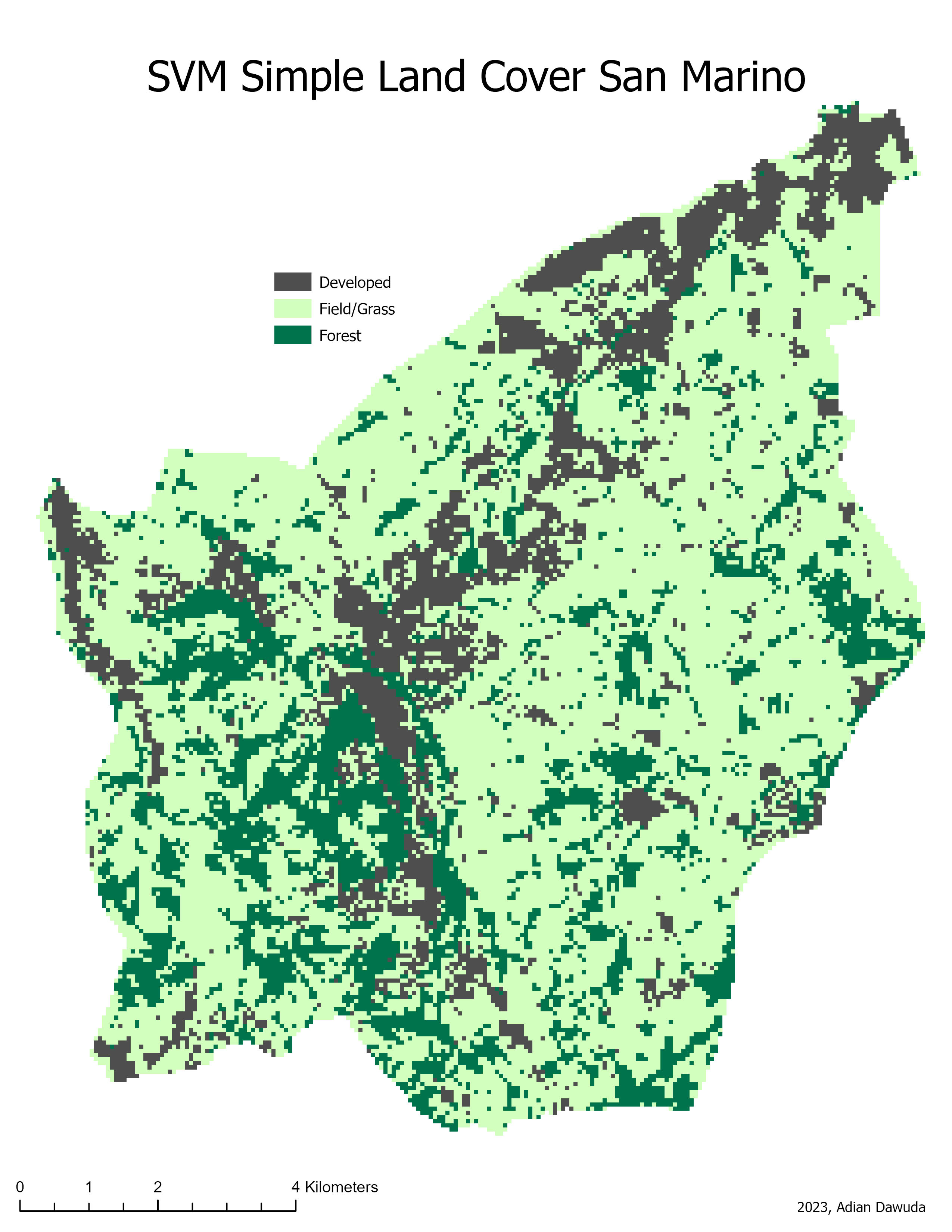
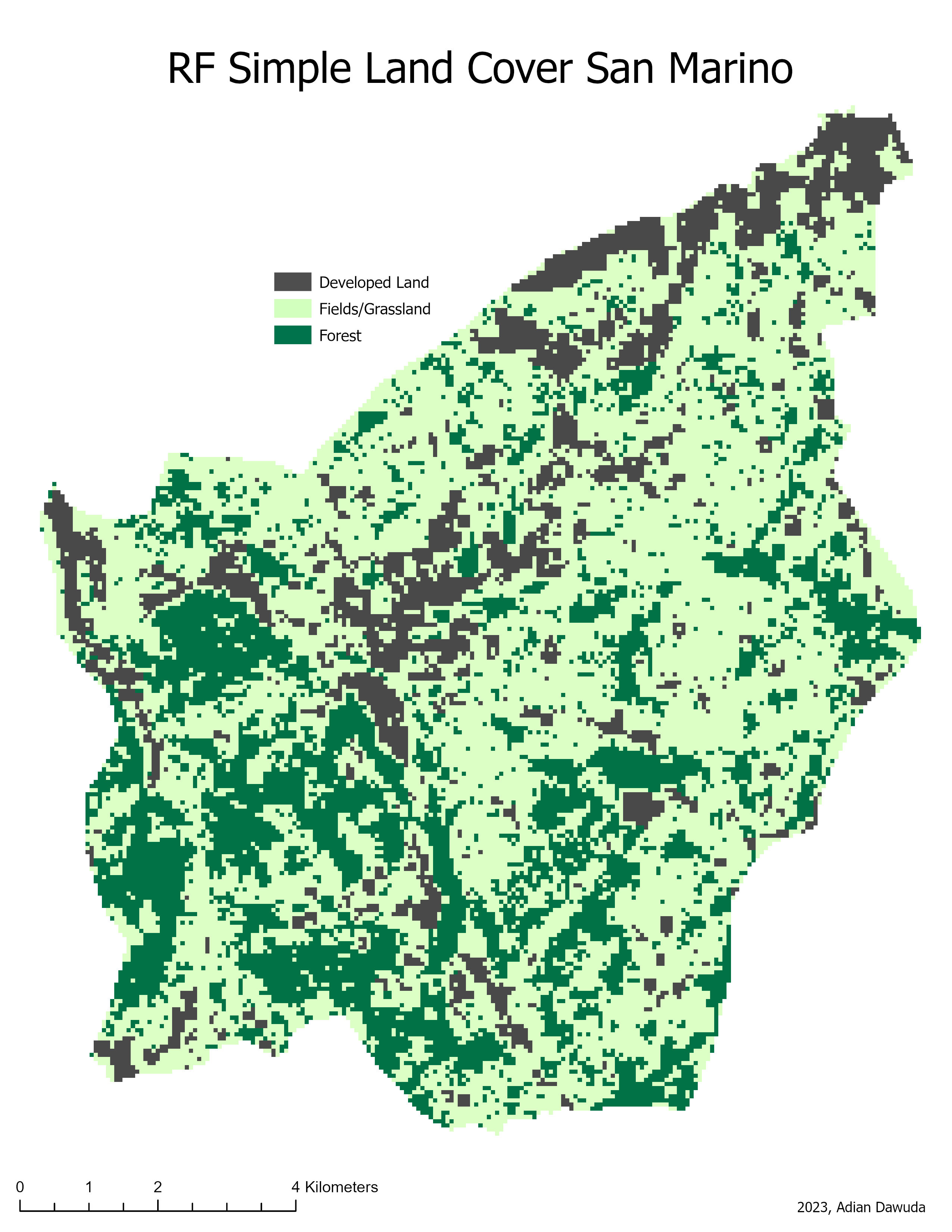
Besides the CLC, which provides a high number of classes with a focus on environmental policy development, a simpler land cover comprising only three classes is created. These three classes are:

• Developed land
• Fields/Grassland
• Forest

The performance of the SVM and RF algorithms will be assessed and compared to each other for both reference classifications.

2.3.2   Satellite Imagery #

The remote sensing imagery analyzed in this project is captured by the European Sentinel-2 satellite, which is equipped with a Multi-Spectral Instrument (MSI) payload able to capture 13 spectral bands (European Space Agency, 2013). The type of processed data used is Level-2A. This delivers Bottom-Of-Atmosphere (BOA) reflectance imagery by applying atmospheric correction to Top-Of-Atmosphere (TOA) imagery. Level-2A data also applies a scene classification algorithm to the imagery, which allows for detailed detection of clouds, cloud shadows, and snow (European Space Agency, 2013).

The data is obtained using the Google Earth Engine web interface. The JavaScript code used can be found in the annex for this paper. As one of the goals of this project is to compare SVM and RF classifications to the 2018 CLC mapping, a composite image of San Marino for the year 2018 (January 1, 2018, to December 31, 2018) is created. The scene classification map created by the scene classification algorithm is used to mask out clouds in the composite image. The image is exported at a spatial resolution of 10 meters.

The data is further prepared in ArcGIS Pro. The steps performed can be replicated using the ArcGIS Pro Python API. The code can be found in the annex for this paper. First, the Sentinel-2 image is clipped to the extent of San Marino’s exact country boundaries. Since the resolution among the bands varies (10 meters: B2, B3, B4, B8. 20 meters: B5, B6, B7, B8b, B11, B12. 60 meters: B1, B9, B10) (European Space Agency, 2013), a copy of the raster image with a spatial resolution of 60m is created using Nearest Neighbor interpolation. Another copy containing only the 10-meter spatial resolution bands (Blue, Red, Green, and Near Infrared) is created. The resulting two images are used as the basis for the following classification.

2.4   Classification #

The SVM and RF classification is also conducted using the ArcGIS Pro Python API. The Forest-based Classification and Regression (RF implementation), and Train Support Vector Machine Classifier tools are used.

First, both algorithms are run to classify the 10-meter resolution image into CLC classes. Both the SVM and RF classifiers are supervised machine learning algorithms that require labeled data as training input. Therefore, representative samples for each class are collected and saved to a file. the SVM and RF classifiers are then trained on the image using a maximum of 500 pixels of the labeled data per class. After training the classifiers, they are used to perform the classification of the image. The accuracy is assessed by comparing the classification with a layer of the CLC of San Marino. This is done by randomly selecting 500 pixels within the image and comparing the class values. A confusion matrix of the classification accuracy is then computed. The quality of the RF classification is additionally determined by assessing the OOB error. The same steps as described above are repeated to classify the 60-meter spatial resolution image into CLC classes and evaluate the results.

Secondly, both algorithms are used to classify both Sentinel images into the simple, three-class land cover classification using the same method. As there is no reference database for the simple classification, the accuracy assessment of the SVM and RF classifications is performed manually. This is done by randomly selecting 50 classified pixels and manually assigning them a simple land cover class. Sentinel and Google Maps imagery is used as a reference to accurately assign classes for each pixel. The validation pixels’ classified classes are then compared to the manually assigned classes and a confusion matrix of the classification accuracy is computed.

3   Results #

Table 1 shows the performance metrics of all classifications performed. The overall OOB error is calculated as the weighted average of the OOB errors for each class.

Table 1: Hyperparameters of an intermediate model achieving promising results on the Cologne test set.

	OOB Error	Accuracy	Kappa Index
CLC SVM 10m	―	0.191	0.092
CLC SVM 60m	―	0.396	0.233
CLC RF 10m	78.282	0.164	0.075
CLC RF 60m	55.289	0.371	0.187
Simple SVM 10m	―	0.868	0.746
Simple SVM 60m	―	0.830	0.699
Simple RF 10m	5.283	0.698	0.456
Simple RF 60m	6.812	0.736	0.544

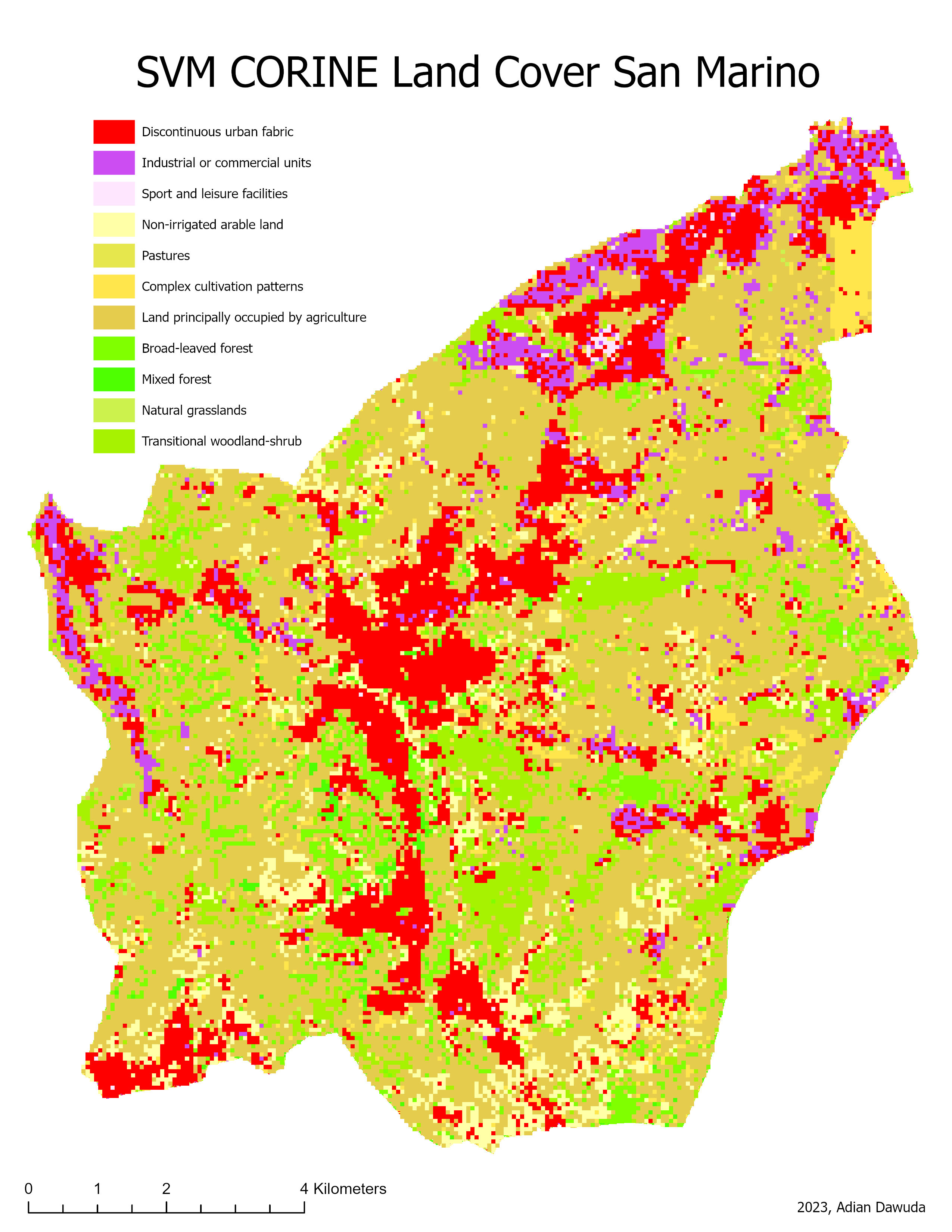
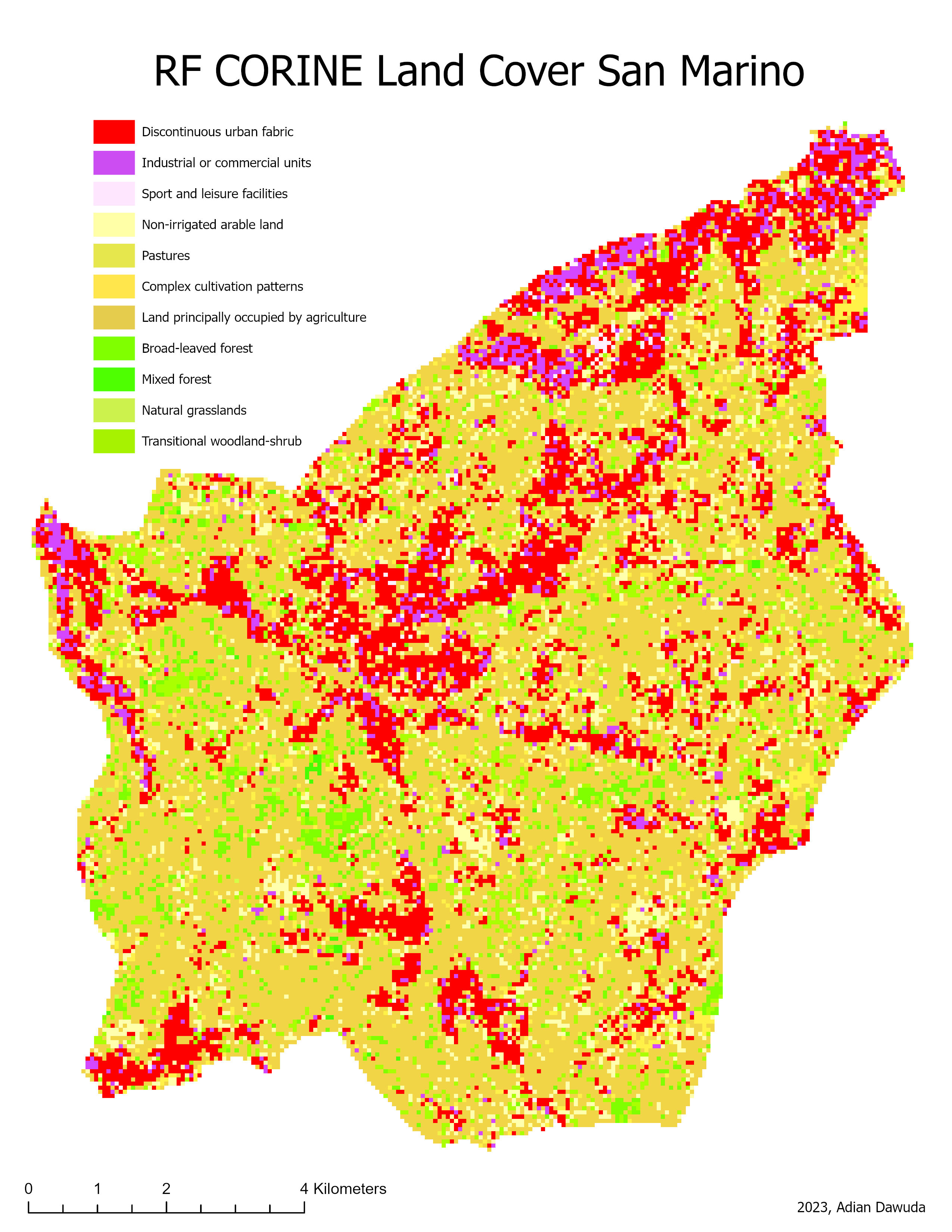
The resulting classifications can be seen in Figures 3 through 10.

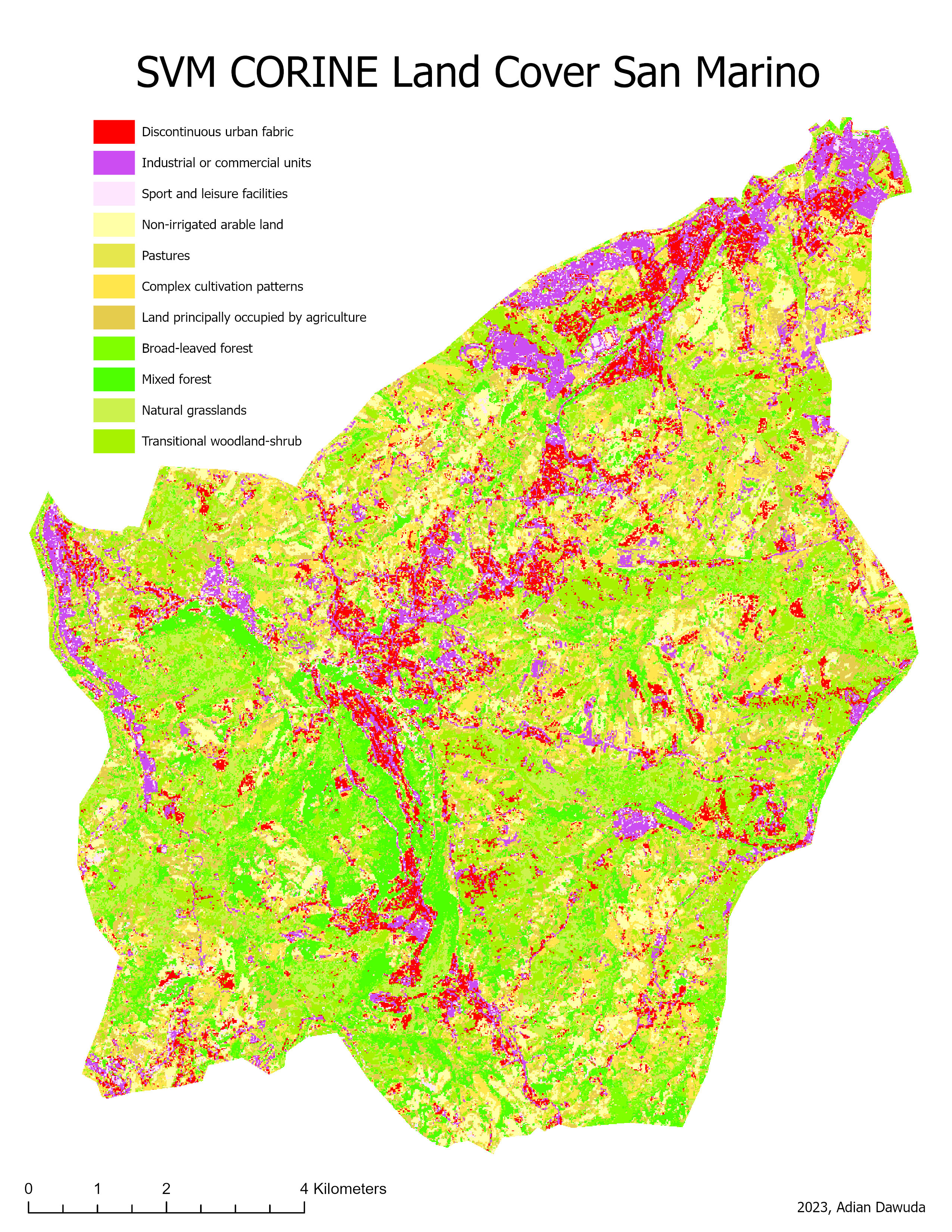
4   Discussion #

For all classifications, the SVM and RF classifiers display comparable visual results and performance metrics. Both the SVM and RF classifiers perform substantially better on the simple land cover than on the CLC. This is confirmed by all evaluation metrics. However, due to only using 50 validation points for the simple land cover accuracy assessment, the statistical significance of the accuracy and Kappa index is lower than for the CLC classification (500 validation points used). Inspecting the accuracy and Kappa index values for all classifications shows that the SVM classifiers slightly outperform the RF classifiers. This aligns with the findings of Thanh Noi & Kappas (2017) and Zhang et al. (2023), where among RF and other machine learning algorithms the SVM achieved the highest land cover classification accuracy.

Decreasing the spatial resolution and increasing the number of bands shows a positive effect on the CLC classification quality for both SVM and RF classifiers. However, for the simple land cover classification no clear improvement is observed. The increased CLC classification quality for the 60m resolution image can be a result of the higher number of available explanatory variables (image bands). This increases the computing power needed but also allows for a clearer distinction between visually (RGB) similar-looking classes. Furthermore, the decreased resolution has a noise-reducing effect. Some CLC classes are quite abstract and contain highly heterogenous pixel values at a high resolution. E.g., Sport and leisure facilities: These may be difficult to correctly classify using a pixel-based approach, as some of the spectral signatures contained in this class are comparable to those contained in built-up or vegetation classes (numerous built-up and vegetation pixels wrongly classified as Sport and leisure facilities, especially in the 10m CLC RF classification). The 10m resolution image, therefore, contains a higher in-class variance of pixel values. At a 60m spatial resolution, this variance is smoothed out, making the class membership of pixels less ambiguous and improving the CLC classification quality. As the spectral signatures of the simple land cover classes have less overlap, the classification quality stays roughly the same at both resolutions.

The CLC also contains classes that may have very similar overall spectral or multispectral signatures, regardless of smoothing, such as Land principally occupied by agriculture, with significant areas of natural vegetation, Broad-leaved forest, Mixed forest, Natural grasslands, and Non-irrigated arable land. The results show that both classification algorithms have trouble correctly assigning the values of these classes. The 10m resolution classifications display a higher amount of forest and grassland classes, while the 60m resolution classifications show higher amounts of agricultural land cover classes. The 10m resolution classifications also misclassify many areas of Discontinuous urban fabric as Industrial or commercial units. The lower resolution classifications create a distinction more closely resembling the CLC reference image.

Overall, the low accuracy of the CLC classifications can be explained by the presence of overlapping pixel values, heterogenous classes, as well as possibly a low number of samples for rare classes like Pastures and Sport and leisure facilities.

The amount of time taken to train the SVM classifier was observed to be significantly longer than for the RF classifier, especially when training the SVM classifier on the CLC. This may be due to the method employed for multiclass classification. As the number of SVMs needed is described by the number of classes \(K\) (OVA classification) or \(K\choose 2\) (OVO classification), either 11 or 55 SVMs need to be trained to classify an image into the CLC classes. It is unclear which method of multiclass classification is employed by the ArcGIS Pro implementation of the SVM algorithm.

To improve the transparency and modularity of the classification process (e.g., choice of SVM kernel and multiclass classification method) in future analyses, lower-level/open implementations of both SVM and RF algorithms should be chosen. The classification quality may be improved by employing an object-based approach with SVM and RF classification, such as the object-based land-cover processing chain employed by Grippa et al. (2017).

5   Conclusion & Outlook #

In conclusion, this project successfully explored the classification of Level-2A Sentinel-2 imagery into CORINE and simple land cover classes using the SVM and RF classifiers. The classifiers were trained and applied on the imagery, and their performance was assessed. Both classifiers achieved comparable results, with the SVM showing slightly higher validation metrics. Both algorithms only achieve a low-accuracy classification for the CLC. The quality of the simple land cover classifications is moderate to high. More modular algorithm implementations and pre-classification image segmentation may improve the results in future analyses.

References #

Belgiu, M., & Drăgu, L. (2016). Random forest in remote sensing: A review of applications and future directions. In ISPRS Journal of Photogrammetry and Remote Sensing (Vol. 114, pp. 24–31). Elsevier B.V. https://doi.org/10.1016/j.isprsjprs.2016.01.011

Breiman, L. (2001). Random Forests. Machine Learning, 45, 5–32.

Büttner, G., Kosztra, B., Maucha, G., Pataki, R., Kleeschulte, S., Hazeu, G., Vittek, M., Littkopf, A., & Schröder, C. (2021). Copernicus Land Monitoring Service. CORINE Land Cover. https://land.copernicus.eu/

Cortes, C., & Vapnik, V. (1995). Support-Vector Networks Editor. In Machine Leaming (Vol. 20). Kluwer Academic Publishers.

Culberg, K., & Fuhs, K. (2017). Feature Extraction in Satellite Imagery Using Support Vector Machines.

Du, P., Samat, A., Waske, B., Liu, S., & Li, Z. (2015). Random Forest and Rotation Forest for fully polarized SAR image classification using polarimetric and spatial features. ISPRS Journal of Photogrammetry and Remote Sensing, 105, 38–53. https://doi.org/10.1016/j.isprsjprs.2015.03.002

European Space Agency. (2013). Sentinel-2 User Handbook.

Grippa, T., Lennert, M., Beaumont, B., Vanhuysse, S., Stephenne, N., & Wolff, E. (2017). An open-source semi-automated processing chain for urban object-based classification. Remote Sensing, 9(4). https://doi.org/10.3390/rs9040358

Hastie, T., Tibshirani, R., & Friedman, J. H. (2009). The elements of statistical learning: data mining, inference, and prediction. Springer.

James, G., Witten, D., Hastie, T., & Tibshirani, R. (2021). An Introduction to Statistical Learning with Applications in R Second Edition.

Kranjčić, N., Medak, D., Župan, R., & Rezo, M. (2019). Support Vector Machine accuracy assessment for extracting green urban areas in towns. Remote Sensing, 11(6). https://doi.org/10.3390/rs11060655

Lang, S., Hay, G. J., Baraldi, A., Tiede, D., & Blaschke, T. (2019). GEOBIA achievements and spatial opportunities in the era of big earth observation data. In ISPRS International Journal of Geo-Information (Vol. 8, Issue 11). MDPI AG. https://doi.org/10.3390/ijgi8110474

Lv, W., & Wang, X. (2020). Overview of Hyperspectral Image Classification. In Journal of Sensors (Vol. 2020). Hindawi Limited. https://doi.org/10.1155/2020/4817234

Mahesh, K. P., Afrouz, S. A., & Areeckal, A. S. (2022). Detection of fraudulent credit card transactions: A comparative analysis of data sampling and classification techniques. Journal of Physics: Conference Series, 2161(1). https://doi.org/10.1088/1742-6596/2161/1/012072

Mammone, A., Turchi, M., & Cristianini, N. (2009). Support vector machines. Wiley Interdisciplinary Reviews: Computational Statistics, 1.3, 283–289. https://doi.org/10.1002/wics.049

Meyer, D. (2009). Support Vector Machines * The Interface to libsvm in package e1071. http://www.csie.ntu.edu.tw/~cjlin/papers/ijcnn.ps.gz.

Murphy, K. P. (2012). Machine learning : a probabilistic perspective.

Pal, M. (2005). Random forest classifier for remote sensing classification. International Journal of Remote Sensing, 26(1), 217–222. https://doi.org/10.1080/01431160412331269698

Rodriguez-Galiano, V. F., Ghimire, B., Rogan, J., Chica-Olmo, M., & Rigol-Sanchez, J. P. (2012). An assessment of the effectiveness of a random forest classifier for land-cover classification. ISPRS Journal of Photogrammetry and Remote Sensing, 67(1), 93–104. https://doi.org/10.1016/j.isprsjprs.2011.11.002

Thanh Noi, P., & Kappas, M. (2017). Comparison of Random Forest, k-Nearest Neighbor, and Support Vector Machine Classifiers for Land Cover Classification Using Sentinel-2 Imagery. Sensors (Basel, Switzerland), 18(1). https://doi.org/10.3390/s18010018

Tzotsos, A. (2006). A SUPPORT VECTOR MACHINE APPROACH FOR OBJECT BASED IMAGE ANALYSIS.

Zhang, C., Liu, Y., & Tie, N. (2023). Forest Land Resource Information Acquisition with Sentinel-2 Image Utilizing Support Vector Machine, K-Nearest Neighbor, Random Forest, Decision Trees and Multi-Layer Perceptron. Forests, 14(2). https://doi.org/10.3390/f14020254