Geodata Acquisition: Photogrammetry Using UAV-Based Aerial Images

This analysis is based on a fictional scenario, where UAV photogrammetry is used to determine whether the goals of a football pitch are equal in size. To do this, images of the pitch are captured and analyzed.

Workflow #

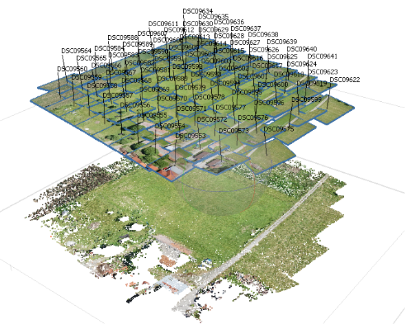
To begin, the UAV images are loaded into the software Agisoft Metashape. Next, the images must be aligned. The Align Photos tool does this by computing tie points and camera positions (Agisoft, 2023) (Figure 1).

Next, the coordinate reference system to be used for the analysis is specified. This is done in the Chunk Reference Settings. The coordinates system is set to MGI / Austria GK Central (EPSG:31255).

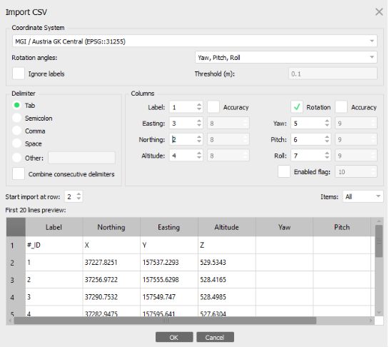
After this, the ground control points (GCPs) are added from a text file (Figure 2). EPSG:31255 is also chosen as the coordinate reference system

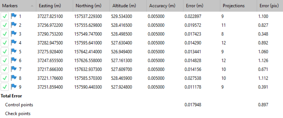
Next, the GCPs are identified manually on as many images as possible, using the provided image that shows the GCP placement for reference. After this, optimization of camera alignment is performed by executing the Optimize Cameras tool (Figure 3). The final accuracy and error of the markers can be seen in Figure 4.

As a next step a point cloud is calculated, which also generates a depth map of the data (Agisoft, 2023). A mesh may be better suited for 3D visualization purposes as the surface is made up of polygons. However, as the goal is to generate an accurate DSM from depth maps, a point cloud is selected. This is also the recommended option by Agisoft when not working with classifications (Agisoft, 2023).

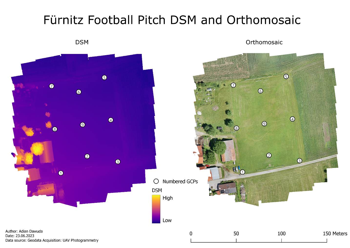
The Build DEM and Build Orthomosaic tools are executed. The Map in Figure 5 shows the calculated DSM and Orthomosaic.

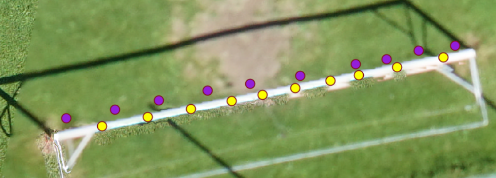
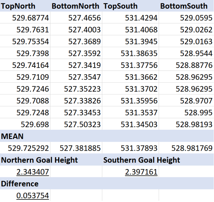
To calculate the difference in height between the goals, 10 samples of the ground and the crossbar are taken at each goal (Figures 6 and 7). In QGIS the Orthomosaic is overlayed to accurately place the points. For each group of samples, the mean elevation is calculated from the DSM. The ground elevation is then subtracted from the crossbar elevation. This produces the mean height of each goal. Because the mean value of multiple samples is used, the influence of outlier measurements is reduced and the result better represents the entirety of each goal. The results (Figure 8) show that the southern goal is roughly 5.4 cm higher than the northern goal.

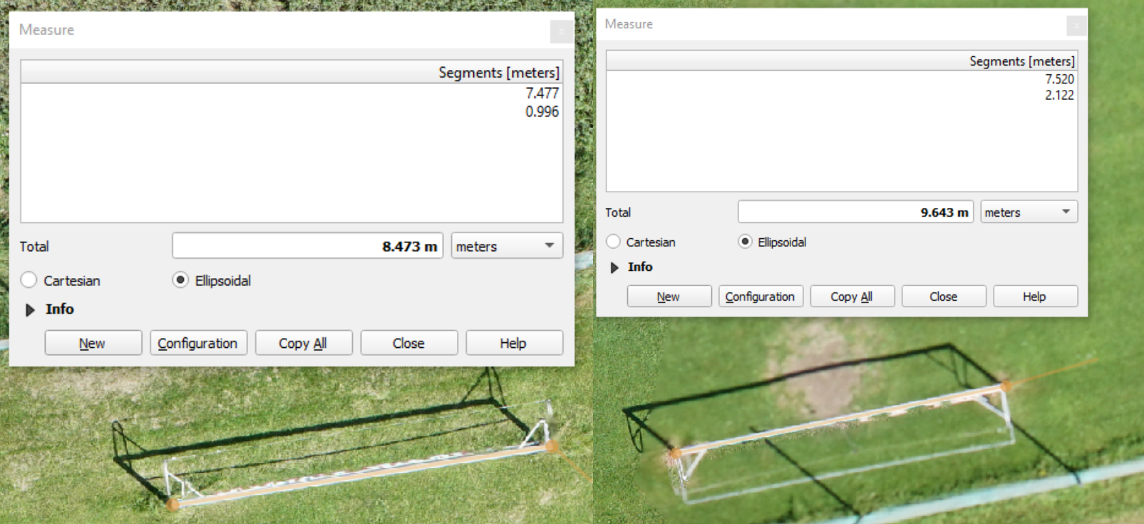
To calculate the difference in the width of the goals, the QGIS Measure tool was used. The results show that the southern goal (7.520 m) is about 4.3 cm wider than the northern goal (7.477 m). This is shown in Figure 9.

Northern Goal = 7.477 × 2.343 = 17.518 m²

Southern Goal = 7.520 × 2.397 = 18.025 m²

Difference = 18.025 − 17.518 = 0.507 m²

Discussion #

The results show that the southern goal is about 0.5 m² larger than the northern goal. Assuming the results represent reality accurately, the effects could very slightly influence a football game. As the differences in height and length are quite small, they may be strongly influenced by measurement inaccuracies. The total error of the GCPs (root mean square of all of the residuals) is roughly 1.8 cm (Figure 4). Given the resolution of the data, the accuracy of most of the results is high. However, the generated orthomosaic contains some blurry portions (e.g., Figure 7). The Seamlines editing option, a different Blending mode, or calculating the orthomosaic from a mesh may be able to fix this (Agisoft, 2023).

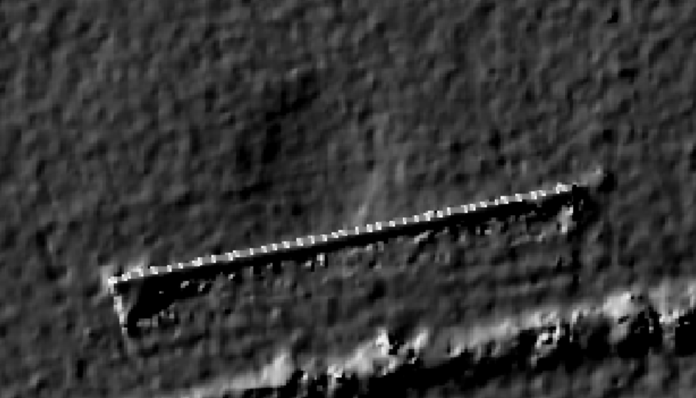
The DSM shows a slight ditch right before the southern goal (Figure 10). This may influence both the measurements and the perceived goal size.

The overall quality of the data is good. The overlap of the images is large enough to find many tie points and the GCPs are easily visible. However, as the differences between the goals range in centimeters, a lower flight path or a higher resolution could have been chosen to minimize measurement errors.

References #

Agisoft. (2023). Agisoft Metashape User Manual Professional Edition, Version 2.0.